Turn the lamp down far enough and light stops pouring. It arrives a grain at a time, each one whole, each landing where no one could have said, and the smooth pictures of the last four chapters build themselves out of chance.
Chapter 5 · Detector
One at a Time
Dim the lamp until light arrives as single clicks. What does a filter do to each one, and how many clicks does a faint pattern need?
Look first
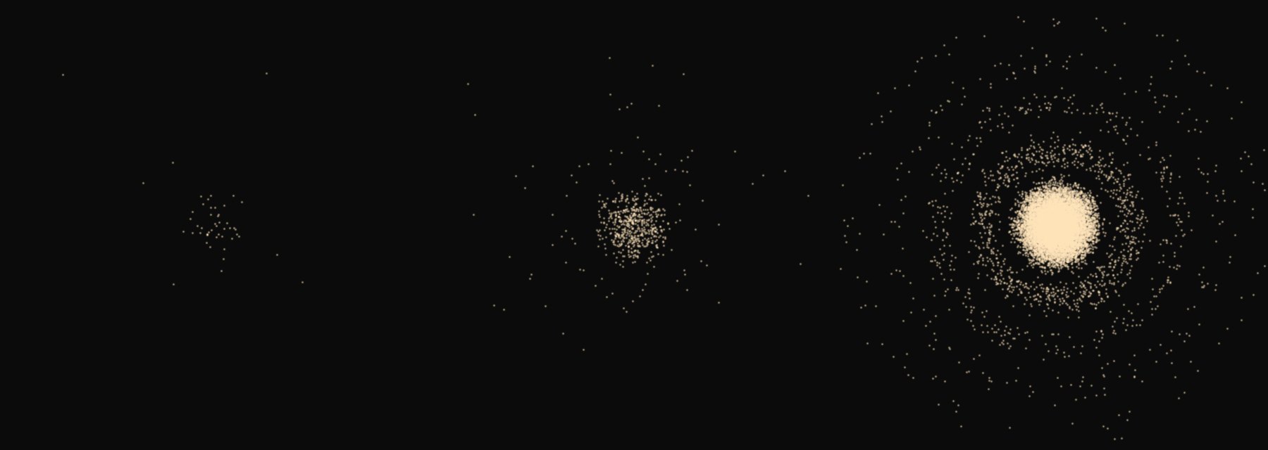
A picture that arrives in grains
This is the image from chapter 1: a distant lamp seen through a pinhole holding two Fresnel zones, the ring with the black centre. But the lamp has been turned down so far that the camera records the light one detection at a time.
At first there is no ring, only scattered points. Each point is a whole detection, the same size as every other. Let them accumulate.
computed
Each detection lands at random, more often where the wave of chapter 1 is bright. 160 × 160 pixels across 0.9 mm.
Commit to a prediction
A quarter of one
Chapter 4 ended here. A polarising filter, then a second one turned 60 degrees from the first. Malus’s law says a quarter of the light gets through: cos²60° = 0.25.
Now the light arrives one detection at a time, as it did in the picture above. A detector after the second filter counts what gets through.
What happens to each arriving detection?
The detections that pass are full size: exactly like the detections with no filter at all. There are simply fewer of them, and nothing about any one of them predicts whether it will pass. Over many, the share comes to a quarter, with a scatter of about four either way in each hundred.
Malus’s law survives, but it has changed what it is about. It no longer says how much of each one gets through. It says how likely each one is to get through.
Why the first guess made sense
The wave is right about the average
If you chose A, you were using the picture that has carried this whole exhibition: light as a smooth wave that a filter trims. For a bright beam it is exactly right, and it still gives the right average here. What it cannot give is a quarter of a click. Detectors never record one.
If you chose C, you were right that the share is fixed. But there is no rhythm to it. A run of five in a row can pass, or none in twenty.
So the wave calculations of chapters 1 to 4 were never pictures of where light goes. They are pictures of where it is likely to be found. Each detection lands whole, at a place, or passes a filter whole, by chance; the wave says how the chances are shared out. The ring with the black centre is real, but it exists only in the accumulation.
The cost: counting noise
Chance has a price. If a pixel should receive, on average, a hundred detections, it actually receives somewhere around a hundred, give or take about ten: the square root of a hundred. With ten thousand it is ten thousand give or take a hundred. The scatter grows more slowly than the count, so the picture gets cleaner as detections pile up, but only slowly.
A faint pattern has to rise above that scatter. The difference between a bright stripe and a dark one grows in proportion to the count. The scatter grows only as its square root. So the fainter the pattern, the more detections you need, and the relation is steep.
The bench
A detector and a filter
On the left, choose a pattern and how many detections to collect. On the right, send single detections at a pair of filters and count what passes.
The detector
Stripes are shown contrast-stretched, as a camera’s screen would: the average is mid-grey, and the typical scatter of one pixel spans most of the range.
Two filters
Things to try
- Set the stripes to 7% contrast, the striae of the glowing diatom in chapter 2. Raise the detections until you are sure you can see them.
- Send batches of 100 at 60°. How often is a batch below 20? Above 30?
- Set the angle to 0° and to 90°. Here chance disappears: all pass, or none.
What you can now say
Light is recorded in whole, separate detections. The wave calculation does not say where the next one lands; it says how likely each place is. A pattern exists only in the accumulation, and seeing a pattern of contrast V takes a number of detections that grows as 1/V².
That is the detector’s own limit, and it applies to any instrument. A fluorescent specimen gives so few detections per second that its faintest detail is lost not to the lens but to counting. Halve a pattern’s contrast and you need four times as long to see it.
For the determined reader: counting statistics, a worked case, and its limits
The quantities
| Symbol | Meaning | Unit |
|---|---|---|
| N | mean number of detections in a pixel | counts |
| V | contrast of the pattern: (bright − dark)/(bright + dark) | none |
| M | number of pixels that share the pattern | none |
| φ | angle between two polarising filters | degrees |
The rules
Independent detections at a steady mean rate give a Poisson count: variance equal to the mean, so a scatter of √N. A filter passing each detection with probability p = cos²φ gives a binomial count from n arrivals: mean np, scatter √(np(1 − p)).
one bright and one dark pixel: signal 2VN, noise √(2N), ratio V√(2N)
M pixels used together: noise on the measured contrast ≈ √(2/(MN))
Either way the detections needed for a given confidence grow as 1/V². For one bright and one dark pixel to pass a one-sided 95% test in 90% of trials needs N ≈ (1.64 + 1.28)²/(2V²).
A worked case
| Contrast V | Needed per pixel (one pair) | Simulated |
|---|---|---|
| 0.07 | 874 | 864 |
| 0.035 | 3,496 | 3,454 |
A whole image does far better than one pair of pixels, because the eye pools many of them along each stripe: in a 64 × 64 image, 7% stripes stand clear of the noise with a few detections per pixel. The absolute numbers depend on how many pixels you pool. The ratio does not. That is why the case you have not seen asks about the ratio.
Where the model stops
It assumes ideal detectors that record every arrival, with no false counts. A real detector records only a fraction (the quantum efficiency), which multiplies the time needed; cameras add read noise, and photomultipliers add dark counts. It assumes detections independent of one another, which holds for lamps, the Sun and fluorescence when counted over times much longer than the light’s coherence time.
The dispute
In the light, or in the detector?
Grainy detections do not, on their own, prove that light comes in grains. A detector might be grainy itself, made of atoms that each respond all at once when enough energy has soaked into them from a perfectly smooth wave. Such a semiclassical picture, smooth light and lumpy detectors, accounts for a surprising amount: the clicks themselves, the photoelectric effect, and fringes that build up dot by dot.
So famous experiments did less than they are often said to. In 1909 G. I. Taylor photographed the shadow of a needle in light so feeble that the exposures ran for months, and the fringes were as sharp as ever. It is a lovely result, but it was done with ordinary light from a flame, and as Grangier, Roger and Aspect pointed out in 1986, ordinary light cannot tell the two pictures apart, however dim.
Their experiment could. They used atoms that emit light in pairs: the first of a pair announced that a second was on its way. Each announced second one went to a half-silvered mirror, with a detector on each side. A smooth wave, however weak, splits at such a mirror and can trigger both detectors at once by chance; there is a floor below which such coincidences cannot fall. Over five hours the wave picture required at least about fifty. They counted nine.
The light really was arriving in whole pieces, each found on one side or the other, never both. Then, with the same source, they built an interferometer around the same mirror. One piece at a time, the fringes appeared, with a contrast above 98%. Asked which way it went, each piece answered one way. Set up so that the question could not be asked, the pieces built fringes, as if each had gone both ways.
A case you have not seen
Half the contrast
The glowing diatom of chapter 2. Its striae come through the lens at 7% contrast. With 20 detections per pixel, on average, you can just make them out across the image.
Now change to a lens that delivers them at half that contrast, 3.5%.
How many detections per pixel to see them as clearly as before?
Lean back from the screen, or squint: your eye pools the pixels along each stripe.
Half the contrast halves the difference between bright and dark stripes. To get it back above the scatter you need to double the ratio of signal to noise, and that ratio grows only as the square root of the count. Doubling a square root takes four times the count.
If you chose B, you reasoned about the signal alone: half as much, so collect twice as long. That would be right if the scatter stayed fixed. It does not; it grows with the count too, only more slowly.
Where this explanation stops
The detector you are using now
Your eye is a detector too. In 1942 Selig Hecht, Simon Shlaer and Maurice Pirenne measured the weakest flash a dark-adapted person can see: between 54 and 148 quanta of blue-green light arriving at the eye. Allowing for what the cornea reflects, the eye’s fluids absorb, and the retina lets through, at most 5 to 14 are absorbed by rods, spread across about 500 of them. So each rod involved absorbs a single quantum. From how often people saw flashes near threshold, they estimated that 5 to 8 such events are needed for a flash to be seen.
In 1979 Denis Baylor and colleagues recorded the electrical current of single rods from a toad’s retina. A single photon produced a clear, discrete response of about one picoampere, the same size at every colour. About half of the photons a rod absorbed produced one.
If a rod can register one photon, why does it take several before a person sees anything? Where, between the rod and the report, does the physics stop and the seeing begin?
End of chapter 5
Added to your notebook
Light is recorded in whole, separate detections; the wave says how likely each place is. Seeing a pattern of contrast V takes detections in proportion to 1/V².
If a rod can register one photon, where does seeing begin?
Chapter 6 · The Last Instrument